Introduction to Data Science with RStudio: A Beginner’s Guide

Play Text-to-Speech:

Data science is an interdisciplinary domain that empowers us to extract valuable insights and knowledge from vast amounts of data. By combining elements from statistics, computer science, and domain expertise, data science enables us to make informed decisions and predictions based on data-driven evidence.

In this guide, we will start by understanding the essence of data science and its role in various industries. We will explore the data science workflow, from data collection and cleaning to data analysis and model building. Throughout the journey, we will focus on using RStudio—an intuitive and popular integrated development environment for the R programming language.

RStudio’s robust capabilities and integration with R’s extensive package ecosystem make it an ideal platform for data manipulation, visualization, and statistical analysis. We will learn how to harness the power of RStudio to perform data cleaning, visualize data trends, and build predictive models.

Table of Contents:

1. Introduction
   1.1 What is Data Science?
   1.2 Why RStudio for Data Science?
   1.3 Setting Up RStudio Environment
2. Basics of R Programming
   2.1 Installing R and RStudio
   2.2 RStudio Interface Overview
   2.3 Basic R Syntax and Data Types
   2.4 Variables and Data Structures
3. Data Import and Export in RStudio
   3.1 Reading and Writing Data Files
   3.2 Dealing with Different Data Formats (CSV, Excel, etc.)
   3.3 Data Inspection and Summary
4. Data Manipulation in RStudio
   4.1 Subsetting and Filtering Data
   4.2 Data Transformation and Reshaping
   4.3 Combining and Merging Data
5. Data Visualization with ggplot2
   5.1 Introduction to Data Visualization
   5.2 Creating Basic Plots with ggplot2
   5.3 Customizing Plots and Adding Visual Enhancements
6. Basic Statistical Analysis with RStudio
   6.1 Descriptive Statistics
   6.2 Hypothesis Testing
   6.3 Correlation and Regression Analysis
7. Introduction to Machine Learning in RStudio
   7.1 What is Machine Learning?
   7.2 Supervised and Unsupervised Learning
   7.3 Building Simple Machine Learning Models
8. Data Science Projects in RStudio
   8.1 Understanding the Data Science Workflow
   8.2 Identifying a Data Science Project
   8.3 Applying Data Science Techniques to Solve Real-world Problems
9. Data Science Resources and Further Learning
   9.1 R and Data Science Communities
   9.2 Online Tutorials and Courses
   9.3 Recommended Books and Blogs
10. Conclusion
    10.1 Recap of Key Concepts
    10.2 Next Steps in Your Data Science Journey

1. Introduction

In the era of big data and advanced technologies, data science has emerged as a crucial discipline that helps organizations and individuals make data-driven decisions and gain valuable insights from vast amounts of data. Data science combines various techniques, tools, and methodologies to extract meaningful information and patterns from raw data.

1.1 What is Data Science?

Data science is an interdisciplinary field that involves using scientific methods, algorithms, and processes to extract knowledge and insights from structured and unstructured data. It combines elements from statistics, mathematics, computer science, domain knowledge, and data engineering. Data scientists collect, clean, and analyze data to uncover hidden patterns, trends, and correlations, which are then used to make informed decisions and predictions.

The data science workflow typically includes:

1. Data Collection: Gathering data from various sources, such as databases, APIs, websites, and sensors.
2. Data Cleaning: Preparing the data for analysis by handling missing values, outliers, and inconsistencies.
3. Data Exploration: Exploring the data through summary statistics and data visualization to gain initial insights.
4. Data Analysis: Applying statistical and machine learning techniques to identify patterns and relationships in the data.
5. Model Building: Creating predictive models using machine learning algorithms.
6. Model Evaluation: Assessing the performance of the models and fine-tuning them for better accuracy.
7. Communication of Results: Presenting the findings and insights to stakeholders in a clear and actionable manner.

1.2 Why RStudio for Data Science?

RStudio is a popular integrated development environment (IDE) for R, a powerful programming language widely used for statistical computing and data analysis. It provides a user-friendly interface, making it easier for data scientists and analysts to work with data and develop analytical solutions. Here are some reasons why RStudio is a preferred choice for data science:

1. Robust Data Analysis: R has a vast collection of packages and libraries that offer a wide range of statistical and data manipulation tools. These packages make data analysis efficient and straightforward.
2. Data Visualization: RStudio’s integration with the ggplot2 package allows data scientists to create high-quality visualizations and graphs with ease, helping them understand data patterns and trends quickly.
3. Reproducibility: RStudio facilitates the creation of reproducible analyses, ensuring that others can replicate your work and validate the results.
4. Data Manipulation: R offers extensive capabilities for data wrangling and transformation, enabling data scientists to clean and preprocess data efficiently.
5. Community Support: The R community is active and vibrant, providing a wealth of resources, tutorials, and help for R users.
6. Integration with RMarkdown: RStudio supports RMarkdown, a tool that allows data scientists to combine code, results, and narrative text into a single document, making it easier to share analyses and reports.

1.3 Setting Up RStudio Environment

Getting started with RStudio is relatively straightforward. Follow these steps to set up your RStudio environment:

1. Install R: Download and install the latest version of R from the official R website.
2. Install RStudio: Go to the RStudio website and download the appropriate version of RStudio for your operating system (Windows, macOS, or Linux).
3. Open RStudio: Launch RStudio after installation. You will see a user-friendly interface with four panes: Console, Environment, Files, and Plots.
4. Install Packages: RStudio allows you to install packages directly from the CRAN repository. To install a package, use the install.packages("package_name") command in the RStudio console.

You are now ready to start your data science journey with RStudio! In the next sections, we will explore the fundamentals of R programming and data manipulation, and dive into data analysis and visualization using RStudio.

2. Basics of R Programming

2.1 Installing R and RStudio

R is a powerful programming language and software environment widely used in data analysis, statistical computing, and data visualization. To get started with R programming, you’ll need to install both R and RStudio, an integrated development environment (IDE) that provides a user-friendly interface for working with R.

Installing R:

• Visit the official R website (https://www.r-project.org/) and download the latest version of R suitable for your operating system (Windows, macOS, or Linux).
• Follow the installation instructions for your operating system, and complete the installation process.

Installing RStudio:

• Go to the RStudio website (https://posit.co/download/rstudio-desktop/) and download the free version of RStudio Desktop.
• Choose the appropriate version for your operating system and install it following the installation wizard.

2.2 RStudio Interface Overview

Once you have installed R and RStudio, let’s familiarize ourselves with the RStudio interface. When you open RStudio, you’ll see four main panes:

• Source Editor: This is where you write and edit your R code. You can save your scripts as R files for future use.
• Console: The console is where your R code is executed, and you’ll see the results and outputs displayed here.
• Environment and History: This pane provides information about your current R session, including variables, data frames, and functions you’ve created.
• Files, Plots, Packages, and Help: These panes allow you to navigate through your file system, view and manage plots, install and load R packages, and access R documentation and help files.

2.3 Basic R Syntax and Data Types

In R, we use various functions and operators to perform operations and computations. Here are some fundamental elements of R programming:

• Arithmetic Operators: R supports standard arithmetic operators such as addition (+), subtraction (-), multiplication (*), division (/), and exponentiation (^).
• Assigning Variables: You can use the assignment operator <- or = to assign values to variables. For example, x <- 10 or y = “Hello”.
• Data Types: R has several basic data types, including numeric (for numerical values), character (for text and strings), logical (for TRUE/FALSE values), and factors (for categorical data).
• Vectors: Vectors are one-dimensional arrays that can hold multiple values of the same data type. You can create vectors using the c() function.
• Data Frames: Data frames are two-dimensional data structures that store data in rows and columns, similar to a table. They are commonly used for data manipulation and analysis.

2.4 Variables and Data Structures

In R, variables are used to store values that can be used and manipulated throughout your code. Here’s how you can work with variables and common data structures:

• Creating Variables: As mentioned earlier, you can create variables by using the assignment operator <- or =. For example, age <- 30 or name = “John”.
• Accessing Elements in Vectors: You can access individual elements in a vector using square brackets []. For example, my_vector[3] will give you the third element of the vector.
• Basic Operations with Vectors: You can perform basic arithmetic operations on vectors, like addition, subtraction, multiplication, and division.
• Data Frames: Data frames are created using the data.frame() function. They allow you to store data in tabular form with rows and columns, making it easy to work with structured data.

Understanding the basics of R programming, installing R and RStudio, and grasping fundamental R syntax and data types are crucial for getting started with data science using R. Once you become familiar with these concepts, you’ll be ready to explore more advanced topics and embark on exciting data science projects. Happy coding!

3. Data Import and Export in RStudio

Data import and export are essential tasks in data science as they allow you to load external datasets into RStudio for analysis and save your results for further use or sharing. In this article, we will explore the process of reading and writing data files in RStudio. We’ll cover various data formats like CSV and Excel, and learn how to inspect and summarize the data after importing.

3.1 Reading and Writing Data Files

Reading Data Files:
In RStudio, you can read data from various file formats into R using dedicated functions. The most commonly used function is read.table(), which can handle plain text files with columns separated by spaces, tabs, or other delimiters. For CSV files, you can use read.csv() or read.csv2() for files with comma or semicolon as the delimiter, respectively.

Example of reading a CSV file:

# Load data from a CSV file into a variable called 'data'
data <- read.csv("data.csv")

Writing Data Files:
Similarly, RStudio provides functions to save your data to various file formats. To save data to a CSV file, you can use write.csv() or write.csv2().

Example of writing data to a CSV file:

# Save the 'data' variable to a CSV file
write.csv(data, "output_data.csv", row.names = FALSE)

3.2 Dealing with Different Data Formats (CSV, Excel, etc.)

Importing and Exporting Excel Files:
RStudio also supports importing and exporting data from Excel files. The read.xlsx() function from the openxlsx package allows you to read data from an Excel file. To export data to an Excel file, you can use the write.xlsx() function from the same package.

Example of importing and exporting Excel files:

# Import data from an Excel file
library(openxlsx)
data <- read.xlsx("data.xlsx")

# Export data to an Excel file
write.xlsx(data, "output_data.xlsx")

Other Data Formats:
Besides CSV and Excel, RStudio can handle various other data formats, such as JSON, XML, SQL databases, and more. For example, you can use the jsonlite package to work with JSON data and the DBI package to interact with SQL databases.

3.3 Data Inspection and Summary

Summary Statistics:
Once you’ve imported your data, it’s essential to get an overview of its characteristics. RStudio provides functions like summary(), str(), and head() to inspect the data. The summary() function gives you summary statistics for each column, while str() displays the structure of the data frame. The head() function shows the first few rows of the dataset.

Example of data inspection:

# Summary statistics
summary(data)

# Structure of the data
str(data)

# First few rows
head(data)

Data Visualization for Inspection:
Visualizing the data can provide valuable insights into its distribution and patterns. Utilize RStudio’s data visualization capabilities, such as ggplot2, to create plots like histograms, box plots, and scatter plots.

Example of data visualization:

# Load the ggplot2 library
library(ggplot2)

# Histogram of a numeric variable
ggplot(data, aes(x = numeric_column)) + geom_histogram()

# Box plot of a numeric variable by a categorical variable
ggplot(data, aes(x = categorical_column, y = numeric_column)) + geom_boxplot()

Data import and export are fundamental tasks in data science using RStudio. By mastering the techniques to read and write data files and understanding data inspection and summary, you lay a strong foundation for your data analysis journey. With RStudio’s flexibility and numerous packages, you can handle various data formats and effectively analyze datasets of different types and sizes.

4. Data Manipulation in RStudio

Data manipulation is a crucial aspect of data science, and RStudio provides powerful tools and functions to manipulate and transform data. In this section, we will explore various techniques for data manipulation using RStudio.

4.1 Subsetting and Filtering Data

Subsetting and filtering data involve extracting specific subsets of data based on certain conditions. In RStudio, you can achieve this using various functions, such as square brackets ([ ]) or the subset() function. Let’s look at some examples:

Example 1: Subsetting Rows Based on Condition

# Create a sample data frame
data <- data.frame(
  Name = c("Alice", "Bob", "Charlie", "David", "Eva"),
  Age = c(25, 30, 22, 27, 28),
  Score = c(85, 78, 92, 80, 88)
)

# Subsetting rows where Age is greater than 25
subset_data <- data[data$Age > 25, ]
print(subset_data)

Output:

    Name Age Score
1  Alice  25    85
2    Bob  30    78
4  David  27    80
5    Eva  28    88

Example 2: Subsetting Columns

# Subsetting columns 'Name' and 'Score'
subset_data <- data[, c("Name", "Score")]
print(subset_data)

Output:

     Name Score
1   Alice    85
2     Bob    78
3 Charlie    92
4   David    80
5     Eva    88

4.2 Data Transformation and Reshaping

Data transformation involves modifying the structure of the data to make it suitable for analysis or visualization. RStudio offers various functions like mutate(), select(), and arrange() for data transformation. Additionally, reshaping data from wide to long or vice versa can be done using functions like gather() and spread(). Let’s see some examples:

Example 1: Data Transformation with mutate()

# Add a new column 'Pass' based on the Score
data <- data %>% 
  mutate(Pass = ifelse(Score >= 80, "Pass", "Fail"))

print(data)

Output:

     Name Age Score Pass
1   Alice  25    85 Pass
2     Bob  30    78 Fail
3 Charlie  22    92 Pass
4   David  27    80 Pass
5     Eva  28    88 Pass

Example 2: Reshaping Data with gather()

# Reshape data from wide to long format
library(tidyr)

wide_data <- data.frame(
  Name = c("Alice", "Bob", "Charlie"),
  Math = c(85, 78, 92),
  Science = c(80, 85, 88)
)

long_data <- gather(wide_data, Subject, Score, Math:Science)

print(long_data)

Output:

     Name Subject Score
1   Alice    Math    85
2     Bob    Math    78
3 Charlie    Math    92
4   Alice Science    80
5     Bob Science    85
6 Charlie Science    88

4.3 Combining and Merging Data

Combining and merging data is essential when you have data distributed across multiple sources or datasets. RStudio offers functions like merge() and bind_rows() to achieve this. Let’s see some examples:

Example 1: Combining Data Frames

# Create two sample data frames
data1 <- data.frame(
  ID = c(1, 2, 3),
  Age = c(25, 30, 22)
)

data2 <- data.frame(
  ID = c(4, 5, 6),
  Age = c(27, 28, 24)
)

# Combine data frames using bind_rows()
combined_data <- bind_rows(data1, data2)

print(combined_data)

Output:

  ID Age
1  1  25
2  2  30
3  3  22
4  4  27
5  5  28
6  6  24

Example 2: Merging Data Frames

# Create two sample data frames
data1 <- data.frame(
  ID = c(1, 2, 3),
  Age = c(25, 30, 22),
  Score = c(85, 78, 92)
)

data2 <- data.frame(
  ID = c(2, 3, 4),
  Height = c(165, 170, 175)
)

# Merge data frames based on ID
merged_data <- merge(data1, data2, by = "ID")

print(merged_data)

Output:

  ID Age Score Height
1  2  30    78    165
2  3  22    92    170

Data manipulation in RStudio is a powerful skill that allows you to extract, transform, and combine data efficiently for further analysis and insights. The examples provided demonstrate some basic operations, and there are many more functions and techniques available in R to handle diverse data manipulation tasks.

5. Data Visualization with ggplot2

Data visualization is a crucial aspect of data science, as it helps to communicate insights and patterns effectively. ggplot2 is a popular data visualization package in RStudio that provides a powerful and flexible system for creating visually appealing and informative plots. In this section, we will explore the basics of data visualization with ggplot2, including creating basic plots and customizing them to enhance their visual impact.

5.1 Introduction to Data Visualization

Data visualization is the representation of data in graphical or visual forms, such as charts, graphs, and maps, to help viewers understand the patterns, trends, and relationships present in the data. It is an essential step in the data analysis process, as it allows data scientists to explore and communicate complex information more effectively than raw numbers or tables.

Data visualization serves several key purposes:

a. Exploratory Data Analysis (EDA): Visualizations help data scientists understand the underlying distribution, outliers, and relationships between variables in the dataset.

b. Presentation and Communication: Well-designed visualizations make it easier to communicate findings to stakeholders, clients, or a broader audience.

c. Pattern Identification: Visual patterns in the data, like trends and clusters, can be more easily identified through graphs and charts.

d. Insight Generation: Visualizations can lead to new insights and hypotheses that might not be apparent from raw data.

5.2 Creating Basic Plots with ggplot2

ggplot2 follows the grammar of graphics, a declarative approach to creating visualizations. It allows you to map data to visual elements, such as points, lines, and bars, and customize the appearance of the plot using layers. Let’s explore how to create some basic plots using ggplot2.

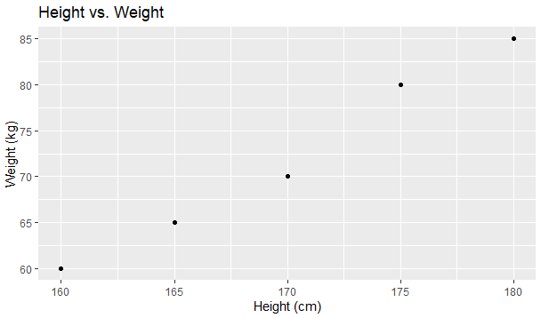
Example: Scatter Plot

A scatter plot is used to visualize the relationship between two continuous variables. Suppose we have a dataset that contains information about the height and weight of individuals:

# Load ggplot2 library
library(ggplot2)

# Sample dataset
data <- data.frame(
  height = c(160, 170, 165, 175, 180),
  weight = c(60, 70, 65, 80, 85)
)

# Create a scatter plot
ggplot(data, aes(x = height, y = weight)) +
  geom_point() +
  labs(title = "Height vs. Weight", x = "Height (cm)", y = "Weight (kg)")

Output:

5.3 Customizing Plots and Adding Visual Enhancements

ggplot2 provides extensive customization options to make plots more visually appealing and informative. You can modify various aspects of the plot, such as axes, colors, labels, and annotations.

Example: Customizing a Bar Plot

Let’s consider a dataset that contains information about the number of products sold in different categories:

# Sample dataset
sales_data <- data.frame(
  category = c("Electronics", "Clothing", "Books", "Furniture"),
  sales = c(120, 80, 150, 90)
)

# Create a bar plot
ggplot(sales_data, aes(x = category, y = sales, fill = category)) +
  geom_bar(stat = "identity") +
  labs(title = "Product Sales by Category", x = "Category", y = "Sales") +
  theme_minimal() +
  theme(axis.text.x = element_text(angle = 45, hjust = 1))

Output:

In this example, we customized the bar plot by changing the theme to a minimal style and rotating the x-axis labels for better readability.

By experimenting with various ggplot2 functions and arguments, you can create a wide range of data visualizations, such as line charts, box plots, histograms, and more. The key is to use the flexibility of ggplot2 to effectively communicate insights from your data.

In the above examples, we used simple datasets for illustrative purposes. In real-world scenarios, data visualization often involves more complex datasets, and ggplot2 provides the flexibility to handle such data effectively and create more insightful visualizations. Remember to install and load the ‘ggplot2’ library before running the code snippets.

6. Basic Statistical Analysis with RStudio

Statistical analysis is a crucial component of data science, as it helps us understand the data, identify patterns, and draw meaningful conclusions. In this section, we will explore some fundamental concepts of statistical analysis using RStudio, a powerful tool for statistical computing and data visualization. We will cover descriptive statistics, hypothesis testing, as well as correlation and regression analysis.

6.1 Descriptive Statistics

Descriptive statistics provides a summary of the main features of a dataset. It allows us to describe and understand the basic properties of the data, such as central tendency, variability, and distribution. Some common descriptive statistics include mean, median, standard deviation, and percentiles.

Example: Calculating Descriptive Statistics

Let’s consider a dataset of students’ exam scores in a mathematics class. We will use RStudio to calculate basic descriptive statistics for this dataset.

# Sample dataset of students' exam scores
exam_scores <- c(85, 78, 92, 65, 88, 75, 90, 82, 79, 95)

# Calculate mean, median, and standard deviation
mean_score <- mean(exam_scores)
median_score <- median(exam_scores)
sd_score <- sd(exam_scores)

# Print the results
print(paste("Mean:", mean_score))
print(paste("Median:", median_score))
print(paste("Standard Deviation:", sd_score))

The output will be:

[1] "Mean: 83"
[1] "Median: 83.5"
[1] "Standard Deviation: 8.5957671098767"

6.2 Hypothesis Testing

Hypothesis testing is a statistical method used to make inferences about a population based on a sample from that population. It involves setting up two competing hypotheses: the null hypothesis (H0) and the alternative hypothesis (Ha). We collect sample data and use it to determine whether there is enough evidence to reject the null hypothesis in favor of the alternative hypothesis.

Example: One-sample t-test

Suppose we have a sample of students’ test scores and we want to test whether the average test score is significantly different from 80.

# Sample dataset of test scores
test_scores <- c(85, 78, 92, 65, 88, 75, 90, 82, 79, 95)

# Perform one-sample t-test
t_test_result <- t.test(test_scores, mu = 80)

# Print the result
print(t_test_result)

The output will show the test statistic, degrees of freedom, and the p-value. Based on the p-value, we can determine whether we reject or fail to reject the null hypothesis.

One Sample t-test

data:  test_scores
t = 1.0162, df = 9, p-value = 0.3361
alternative hypothesis: true mean is not equal to 80
95 percent confidence interval:
 76.44459 89.35541
sample estimates:
mean of x 
     82.9 

6.3 Correlation and Regression Analysis

Correlation measures the strength and direction of the linear relationship between two continuous variables. It helps us understand how changes in one variable are associated with changes in another variable. Regression analysis, on the other hand, allows us to model and predict the relationship between a dependent variable and one or more independent variables.

Example: Correlation and Linear Regression

Consider a dataset with two variables: hours of study and exam scores. We want to investigate the correlation between study hours and exam scores and perform a linear regression to predict exam scores based on study hours.

# Sample dataset
study_hours <- c(4, 5, 2, 6, 3, 7, 5, 8, 6, 7)
exam_scores <- c(75, 85, 60, 90, 70, 95, 80, 98, 85, 92)

# Calculate the correlation coefficient
correlation <- cor(study_hours, exam_scores)

# Perform linear regression
linear_model <- lm(exam_scores ~ study_hours)

# Print the results
print(paste("Correlation Coefficient:", correlation))
print(summary(linear_model))

The output will show the correlation coefficient between study hours and exam scores, as well as the coefficients of the linear regression model.

[1] "Correlation Coefficient: 0.982505823713784"
Call:
lm(formula = exam_scores ~ study_hours)

Residuals:
    Min      1Q  Median      3Q     Max 
-2.5421 -1.6885 -0.5405  1.4104  3.8598 

Coefficients:
            Estimate Std. Error t value Pr(>|t|)    
(Intercept)  50.1433     2.3243   21.57 2.25e-08 ***
study_hours   6.1994     0.4155   14.92 4.01e-07 ***
---
Signif. codes:  0 ‘***’ 0.001 ‘**’ 0.01 ‘*’ 0.05 ‘.’ 0.1 ‘ ’ 1

Residual standard error: 2.354 on 8 degrees of freedom
Multiple R-squared:  0.9653,	Adjusted R-squared:  0.961 
F-statistic: 222.7 on 1 and 8 DF,  p-value: 4.012e-07

Understanding basic statistical analysis is essential for any data scientist. RStudio provides powerful tools and functions to perform various statistical analyses easily and efficiently. By mastering descriptive statistics, hypothesis testing, and correlation and regression analysis in RStudio, you can gain valuable insights from your data and make data-driven decisions with confidence.

7. Introduction to Machine Learning in RStudio

In this section, we delve into the exciting world of machine learning, a pivotal aspect of data science. Machine learning is the art and science of training computers to learn from data and make predictions or decisions without being explicitly programmed. In the context of RStudio, you’ll find it to be a powerful tool for developing and implementing machine learning models.

7.1 What is Machine Learning?

Machine learning can be seen as a subset of artificial intelligence (AI) that focuses on developing algorithms and statistical models that enable computers to learn and improve their performance on specific tasks through experience. Here are some key concepts:

• Data-Driven Learning: Machine learning algorithms are data-driven. They learn patterns and relationships within the data, allowing them to make predictions or decisions based on new, unseen data.
• Types of Learning: Machine learning can be categorized into three main types: supervised learning, unsupervised learning, and reinforcement learning. Each type serves different purposes:
• Supervised Learning: In supervised learning, the model learns from labeled data, making predictions or classifications based on input-output pairs. It’s like teaching a model by showing it examples and letting it learn from them.
• Unsupervised Learning: Unsupervised learning involves finding patterns or structures in unlabeled data. It is often used for clustering similar data points or reducing the dimensionality of data.
• Reinforcement Learning: Reinforcement learning is about training agents to make sequences of decisions in an environment to maximize a reward. It’s commonly used in robotics and gaming.
• Applications: Machine learning has a wide range of applications, from natural language processing and image recognition to recommendation systems and autonomous vehicles. It plays a crucial role in modern technology and industry.

7.2 Supervised and Unsupervised Learning

Machine learning algorithms can be further categorized into supervised and unsupervised learning methods. Understanding the difference between these two is essential for building machine learning models in RStudio.

• Supervised Learning: In supervised learning, the algorithm is provided with labeled training data. This means that each data point in the training set has a corresponding target or output value. The algorithm’s goal is to learn a mapping from inputs to outputs. Common supervised learning algorithms include linear regression, decision trees, and neural networks. Applications include image classification, spam email detection, and predicting house prices.
• Unsupervised Learning: Unsupervised learning, on the other hand, deals with unlabeled data. The algorithm tries to find patterns, structures, or relationships within the data without any predefined targets. Common unsupervised learning techniques include clustering (e.g., k-means) and dimensionality reduction (e.g., PCA). Applications include customer segmentation and anomaly detection.

7.3 Building Simple Machine Learning Models

Now that you have a foundational understanding of machine learning, it’s time to dive into the practical aspect of building simple machine learning models in RStudio. Here are the general steps involved:

1. Data Preparation: Clean, preprocess, and format your data. This includes handling missing values, scaling features, and splitting the data into training and testing sets.
2. Model Selection: Choose an appropriate machine learning algorithm based on the nature of your problem (classification, regression, etc.) and the characteristics of your data.
3. Model Training: Feed the training data into the chosen algorithm to train the model. During training, the algorithm learns the patterns and relationships in the data.
4. Model Evaluation: Assess the model’s performance using evaluation metrics such as accuracy, precision, recall, and F1-score (for classification) or mean squared error (for regression).
5. Hyperparameter Tuning: Fine-tune the model by adjusting hyperparameters to optimize its performance.
6. Deployment: Once satisfied with the model’s performance, deploy it to make predictions on new, unseen data.

As you delve deeper into machine learning with RStudio, you’ll encounter various libraries and packages such as caret, randomForest, and xgboost, which simplify the process of model building and evaluation.

Let’s dive into using the caret package in RStudio for machine learning. The caret (Classification And REgression Training) package is a versatile tool that simplifies the process of building, evaluating, and comparing machine learning models. It provides a unified interface to various machine learning algorithms and streamlines tasks like data preprocessing and model tuning. Here’s a simple example using the caret package for a classification task:

Example: Classification with caret

In this example, we’ll use the famous Iris dataset for a basic classification task. We aim to predict the species of iris flowers based on their sepal length, sepal width, petal length, and petal width.

First, make sure you have the caret package installed. If not, you can install it using:

install.packages("caret")

Now, let’s proceed with the example:

# Load the required libraries
library(caret)
library(e1071)  # We'll use the SVM algorithm from the e1071 package

# Load the Iris dataset
data(iris)

# Split the data into training and testing sets (70% training, 30% testing)
set.seed(123)  # For reproducibility
trainIndex <- createDataPartition(iris$Species, p = 0.7, 
                                  list = FALSE, 
                                  times = 1)
trainData <- iris[ trainIndex,]
testData <- iris[-trainIndex,]

# Define the training control
ctrl <- trainControl(method = "cv",   # 10-fold cross-validation
                     number = 10,     # Number of folds
                     classProbs = TRUE)  # Save class probabilities

# Train a Support Vector Machine (SVM) model
svm_model <- train(Species ~ ., 
                   data = trainData, 
                   method = "svmRadial",  # Radial basis kernel SVM
                   trControl = ctrl)

# Print the model
svm_model

In this example, we:

1. Load the caret and e1071 packages.
2. Load the Iris dataset and split it into training and testing sets.
3. Define the training control using 10-fold cross-validation.
4. Train a Support Vector Machine (SVM) model using the radial basis kernel.

After running this code, you’ll have a trained SVM model. You can then use this model to make predictions on new data and evaluate its performance on the test set. caret makes it easy to switch between different algorithms and tune their hyperparameters using a consistent interface.

Remember to adjust the method and parameters based on your specific problem and dataset. This is just a basic example to get you started with caret for classification in RStudio.

8. Data Science Projects in RStudio

In this section, we’ll explore the essential aspects of data science projects in RStudio. Data science projects involve a systematic approach to solving real-world problems using data-driven techniques. Whether you’re a beginner or an experienced data scientist, understanding the workflow, project identification, and application of data science techniques is crucial for success.

8.1 Understanding the Data Science Workflow

The data science workflow is a structured process that guides data scientists through the various stages of a project. Here’s an overview of the typical steps:

1. Problem Definition: Begin by clearly defining the problem you want to solve. What is the business or research question? What are the objectives and constraints?
2. Data Collection: Gather relevant data from various sources. This may involve web scraping, data extraction from databases, or using pre-existing datasets.
3. Data Preprocessing: Clean, format, and prepare the data for analysis. This step includes handling missing values, outlier detection, and feature engineering.
4. Exploratory Data Analysis (EDA): Explore the data to gain insights. Use summary statistics, data visualizations, and correlation analysis to understand the dataset’s characteristics.
5. Feature Selection: Identify the most relevant features (variables) for your problem. Feature selection can improve model performance and reduce complexity.
6. Model Building: Choose appropriate machine learning or statistical models based on the nature of your problem (classification, regression, clustering, etc.). Train and evaluate the models using suitable techniques like cross-validation.
7. Model Evaluation: Assess model performance using relevant metrics (accuracy, F1-score, RMSE, etc.). Fine-tune hyperparameters to optimize model performance.
8. Model Interpretability: Understand how the model makes predictions. Visualize feature importance or use techniques like SHAP values to interpret complex models.
9. Deployment: Deploy the model into a production environment if applicable. This step may involve creating APIs or integrating the model into a web application.
10. Monitoring and Maintenance: Continuously monitor model performance in production. Retrain the model with new data as needed. Data science is an iterative process.

8.2 Identifying a Data Science Project

Identifying a suitable data science project is a crucial step. Here’s how you can identify a project:

• Business or Research Need: Look for areas where data-driven insights can make a significant impact. This could be in optimizing business processes, improving customer experiences, or advancing scientific research.
• Data Availability: Ensure that you have access to relevant data. Consider both the quantity and quality of data. Sometimes, data may need to be collected or acquired.
• Clear Objectives: Define clear and measurable objectives. What do you aim to achieve with your project? What are the key performance indicators (KPIs)?
• Feasibility: Assess whether the project is technically feasible with your current skill set and resources. If not, consider seeking additional expertise or tools.
• Value Proposition: Determine the potential value of the project. Will it lead to cost savings, revenue generation, or improved decision-making?

8.3 Applying Data Science Techniques to Solve Real-world Problems

Now, let’s illustrate the application of data science techniques to solve a real-world problem using RStudio. Suppose you’re working on a customer churn prediction project for a telecommunications company. The goal is to identify customers at risk of churning (canceling their subscriptions) so that the company can take proactive measures to retain them.

Here’s a simplified example of the workflow:

1. Problem Definition: Define the problem as “Predicting customer churn based on historical data.”
2. Data Collection: Gather historical customer data, including features like contract type, monthly charges, usage patterns, and customer demographics.
3. Data Preprocessing: Clean the data, handle missing values, and encode categorical variables. Perform feature scaling if necessary.
4. Exploratory Data Analysis (EDA): Explore the data to understand customer behavior. Identify trends and correlations.
5. Feature Selection: Select relevant features based on EDA and domain knowledge.
6. Model Building: Choose classification algorithms (e.g., logistic regression, random forest) and train models on the labeled data.
7. Model Evaluation: Evaluate models using metrics like accuracy, precision, recall, and F1-score. Fine-tune hyperparameters to optimize performance.
8. Model Interpretability: Interpret the model’s predictions to identify key factors influencing churn.
9. Deployment: Deploy the model into the company’s system to predict customer churn in real-time.
10. Monitoring and Maintenance: Continuously monitor model performance and update it as new customer data becomes available.

This example showcases how data science techniques are applied to solve a practical business problem, helping the company reduce customer churn and improve customer retention.

In RStudio, you can use various packages like caret, tidyverse, and ggplot2 to streamline the entire workflow, from data preprocessing to model building and visualization.

9. Data Science Resources and Further Learning

In the ever-evolving field of data science, staying updated and continuously learning is essential. In this section, we will explore valuable resources and avenues for furthering your data science knowledge and skills.

9.1 R and Data Science Communities

Engaging with data science communities can be a rich source of knowledge sharing, networking, and collaboration. Here are some prominent communities for R and data science enthusiasts:

• RStudio Community: The RStudio Community is an active forum where you can ask questions, share insights, and interact with fellow R users and data scientists. It’s a great place to seek help with coding challenges or share your expertise.
• Kaggle: Kaggle is a renowned platform for data science competitions and collaborative data analysis projects. It offers datasets, notebooks, and forums where you can learn from and collaborate with a global community of data scientists.
• Stack Overflow: While not specific to R or data science, Stack Overflow is a valuable resource for solving programming and data-related questions. Many R and data science experts contribute to this platform.

9.2 Online Tutorials and Courses

Online tutorials and courses provide structured learning paths for mastering data science concepts and tools. Here are some recommended platforms and courses:

• Coursera: Coursera offers a wide range of data science courses, including the “Data Science Specialization” by Johns Hopkins University, which covers R programming and machine learning.
• edX: edX provides courses such as “Data Science MicroMasters Program” by UC Berkeley, which includes R-based courses and covers various data science topics.
• DataCamp: DataCamp offers interactive R courses specifically tailored for data science. Their hands-on approach helps you apply what you learn in real projects.
• LinkedIn Learning: LinkedIn Learning has numerous data science courses, including “Data Science Foundations: R Basics” and “Data Science Foundations: Fundamentals.”

9.3 Recommended Books and Blogs

Books and blogs are excellent resources for deepening your understanding of data science principles and techniques. Here are some highly regarded books and blogs in the field:

Books:

• “Introduction to Statistical Learning” by Gareth James, Daniela Witten, Trevor Hastie, and Robert Tibshirani. This book covers essential topics in statistical learning and provides R code examples.
• “R for Data Science” by Hadley Wickham and Garrett Grolemund. This book is an excellent resource for learning R specifically for data science.
• “Python for Data Analysis” by Wes McKinney. While focused on Python, this book is valuable for understanding data manipulation and analysis concepts.

Blogs:

• R-Bloggers: R-Bloggers is a community of R users who contribute articles, tutorials, and insights related to R programming and data science.
• Simply Statistics: The Simply Statistics blog is authored by three biostatistics professors and provides valuable perspectives on data science and statistics.
• Towards Data Science: Towards Data Science is a Medium publication featuring a wide range of data science articles, tutorials, and insights from the community.

These resources should provide a solid foundation for your ongoing learning journey in data science. Remember that the field is dynamic, so staying engaged with the community and continuously exploring new resources is key to your professional growth.

10. Conclusion

As we reach the conclusion of this beginner’s guide to data science with RStudio, it’s essential to reflect on the key concepts you’ve encountered throughout this journey. Data science is a multifaceted field that combines statistical analysis, programming, domain expertise, and a thirst for knowledge to extract meaningful insights from data. In this concluding section, we’ll recap the essential takeaways and outline your next steps in the exciting world of data science.

10.1 Recap of Key Concepts

Throughout this guide, we’ve covered a range of foundational concepts and skills:

• What is Data Science: Data science is the art and science of extracting actionable insights from data. It encompasses data collection, cleaning, analysis, visualization, and the development of predictive models.
• RStudio for Data Science: RStudio is a powerful integrated development environment (IDE) for the R programming language, making it an ideal tool for data analysis and visualization.
• Basics of R Programming: You’ve learned about installing R and RStudio, navigating the interface, and working with R’s syntax and data structures.
• Data Import and Export: We explored methods for reading and writing data in various formats, including CSV and Excel, and how to inspect and summarize data.
• Data Manipulation: Techniques for subsetting, filtering, transforming, and merging data were covered, enabling you to prepare data for analysis effectively.
• Data Visualization: You gained insights into creating visually appealing and informative plots using the ggplot2 package.
• Basic Statistical Analysis: Descriptive statistics, hypothesis testing, and correlation and regression analysis were introduced as fundamental tools for data exploration.
• Introduction to Machine Learning: You were introduced to the world of machine learning, including supervised and unsupervised learning, and the process of building simple machine learning models.
• Data Science Projects: Understanding the data science workflow and how to identify and solve real-world problems using data-driven techniques.
• Data Science Resources: Valuable resources, including online communities, tutorials, courses, books, and blogs, were provided to support your ongoing learning journey.

10.2 Next Steps in Your Data Science Journey

Your journey in data science is just beginning, and there’s a world of opportunities waiting for you. Here are some next steps to consider:

• Specialize: Depending on your interests, consider specializing in a specific area of data science, such as machine learning, natural language processing, or computer vision.
• Projects: Practice your skills by working on real data science projects. This hands-on experience is invaluable for mastering concepts and building a portfolio.
• Advanced Learning: Continue your education with advanced courses, certifications, or degrees in data science or related fields to deepen your knowledge.
• Contribute: Share your knowledge and expertise with the data science community. Consider writing articles, participating in open-source projects, or mentoring others.
• Stay Updated: Data science is a rapidly evolving field. Stay updated with the latest developments, tools, and techniques by following blogs, attending conferences, and reading research papers.
• Network: Connect with other data scientists, attend meetups, conferences, and webinars to expand your professional network.

Remember that learning is an ongoing process, and the journey is as rewarding as the destination. Whether you’re pursuing a career in data science, using data analysis skills in your current role, or simply exploring the field out of curiosity, the knowledge and skills you’ve gained in this guide will serve as a solid foundation for your data science endeavors. Embrace the challenges, keep exploring, and continue your exciting data science journey with enthusiasm and curiosity.