Integrating Weibull Distribution, Inter-Failure Analysis, and Reliability Growth for Engineering Decision-Making

Play Text-to-Speech:

1. Introduction: From Failure Data to Engineering Decisions

In complex industrial environments—whether in power plants, petrochemical facilities, utilities, or rotating equipment systems—failures are not isolated events. They are manifestations of underlying system behavior shaped by design, operation, maintenance practices, and environmental conditions. Engineers responsible for maintaining system performance are not only tasked with restoring operation but also with understanding why failures occur, how they evolve over time, and what actions can prevent recurrence.

Three analytical perspectives are central to this effort: Weibull distribution, inter-failure time (TBF) analysis, and reliability growth modeling. Each represents a different lens through which failure data can be interpreted. Individually, they provide valuable insights. When integrated, they form a powerful framework for transforming raw failure data into actionable engineering decisions.

This article develops a structured, systems-level understanding of these methods, their relationships, and their practical application in reliability engineering.

2. Weibull Distribution: Understanding Failure Mechanisms

The Weibull distribution is widely regarded as the foundational model for analyzing time-to-failure data. Its strength lies in its flexibility to represent different failure behaviors through a single parameter: the shape parameter (β).

The Weibull probability density function is:

2.1 Interpretation of the Shape Parameter (β)

The shape parameter defines the failure behavior:

• β < 1 (Infant Mortality Region)
  Failures are concentrated early in life. Common causes include manufacturing defects, installation errors, or commissioning issues.
• β = 1 (Random Failure Region)
  The failure rate is constant. Failures occur independently of age, often due to external stressors or random disturbances.
• β > 1 (Wear-Out Region)
  Failure rate increases with time. This indicates aging, fatigue, corrosion, or material degradation.

2.2 Engineering Significance

Weibull analysis answers a critical question:

“What is the dominant failure mechanism in the system?”

This insight directly supports:

• Maintenance strategy selection
• Replacement interval optimization
• Root cause analysis (RCA) validation

However, Weibull assumes that each failure represents a complete lifecycle, which is not always valid in real operating systems.

3. Inter-Failure Time (TBF): Observing System Behavior

In operating systems, especially those undergoing repair, engineers often work with inter-failure times rather than complete lifecycles.

Inter-failure time is defined as:

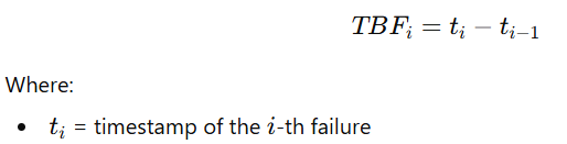
3.1 Nature of TBF Data

Unlike Weibull life data:

• TBF represents intervals between failures
• It captures system-level behavior
• It reflects the combined effect of multiple failure modes

3.2 Limitations of Simple TBF Analysis

A common mistake is to treat TBF as independent and identically distributed data. In reality:

• Repairs may not restore the system to “as good as new”
• Degradation accumulates over time
• Operational conditions may change

Therefore:

• Mean TBF alone is insufficient
• Trend analysis becomes essential

4. Reliability Growth: Understanding System Evolution

Reliability growth analysis addresses a fundamentally different question:

“Is the system becoming more reliable or less reliable over time?”

This is particularly relevant for:

• Systems under continuous operation
• Assets undergoing iterative improvement
• Facilities experiencing recurring failures

4.1 Crow-AMSAA Model (NHPP Power Law)

The most widely used model for reliability growth is the Crow-AMSAA model, expressed as:

4.2 Interpretation of β in Reliability Growth

• β < 1 (Improvement / Growth)
  Failures occur less frequently over time. Corrective actions are effective.
• β = 1 (Random Behavior)
  No improvement or degradation. System operates at steady state.
• β > 1 (Degradation)
  Failures accelerate. Indicates aging, design weakness, or systemic issues.

4.3 Engineering Value

Reliability growth analysis provides:

• Evidence of improvement effectiveness
• Early warning of degradation
• Quantitative support for CAPEX decisions

5. Connecting Weibull, TBF, and Reliability Growth

5.1 Conceptual Integration

Each method addresses a different dimension of reliability:

• Weibull Distribution → Failure Mechanism (Why failures occur)
• TBF Analysis → Failure Pattern (What is happening)
• Reliability Growth → System Trend (Where the system is heading)

Together, they form a complete diagnostic framework.

5.2 Micro vs Macro Perspective

• Weibull operates at the component level
• Crow-AMSAA operates at the system level
• TBF bridges both perspectives

This distinction is critical in complex systems where:

• Multiple failure modes coexist
• Repairs are imperfect
• System behavior evolves over time

6. Practical Engineering Interpretation

6.1 Scenario 1: Early Failures (β < 1)

• Weibull indicates infant mortality
• TBF shows short intervals initially
• Crow-AMSAA β < 1 confirms improvement

Engineering action:

• Improve commissioning practices
• Eliminate design or installation defects

6.2 Scenario 2: Random Failures (β ≈ 1)

• Failures are unpredictable
• TBF shows no clear trend
• Growth model β ≈ 1

Engineering action:

• Enhance monitoring systems
• Introduce redundancy

6.3 Scenario 3: Wear-Out Failures (β > 1)

• Weibull indicates aging
• TBF decreases over time
• Growth model β > 1 confirms degradation

Engineering action:

• Implement preventive replacement
• Justify equipment overhaul or CAPEX

7. Beyond Classical Methods: Advanced Models

7.1 Non-Homogeneous Poisson Process (NHPP)

Generalizes reliability growth models:

• Allows time-varying failure rates
• Suitable for evolving systems

7.2 Renewal Process

Applicable when:

• System is restored to “as good as new” after repair

Bridges Weibull and TBF analysis.

7.3 Proportional Hazard Model (PHM)

Incorporates operating conditions:

Applications:

• Predictive maintenance
• Condition-based monitoring

7.4 Bayesian Reliability Models

Used when:

• Data is limited
• Uncertainty is high

Enables continuous updating as new data becomes available.

8. Engineering Workflow for Integrated Analysis

A structured approach ensures that analysis leads to actionable decisions.

8.1 Step 1: Data Collection

• Failure timestamps
• Operating conditions
• Maintenance actions

8.2 Step 2: TBF Calculation

• Compute inter-failure intervals
• Identify trends

8.3 Step 3: Reliability Growth Analysis

• Fit Crow-AMSAA model
• Determine growth or degradation

8.4 Step 4: Weibull Analysis

• Fit life distribution
• Identify failure mechanism

8.5 Step 5: Decision-Making

• Maintenance strategy selection
• Root cause validation
• CAPEX justification

9. Application in Industrial Systems

Consider a nitrogen generation system experiencing declining performance.

Observed data:

• Increasing failure frequency
• Reduced output capacity
• Instability in operating pressure

Analysis:

• TBF shows decreasing intervals
• Crow-AMSAA β > 1 indicates degradation
• Weibull β > 1 suggests wear-out mechanism

Interpretation:

• System is not experiencing random failures
• Degradation is systematic, possibly due to material fatigue or control instability

Engineering decision:

• Evaluate component replacement (e.g., CMS material)
• Investigate control system mismatch
• Justify capital investment based on reliability decline

10. Strategic Importance in Reliability Engineering

The integration of these methods aligns with international best practices, including:

• Reliability-centered maintenance (RCM)
• MIL-HDBK-189 (Reliability Growth Management)
• IEC reliability standards

These frameworks emphasize:

• Data-driven decision-making
• Continuous improvement
• System-level thinking

11. Common Pitfalls and Misinterpretations

11.1 Over-Reliance on MTBF

• MTBF hides variability and trends
• Does not indicate improvement or degradation

11.2 Misapplication of Weibull

• Using Weibull for repairable systems without validation
• Ignoring dependency between failures

11.3 Ignoring System Context

• Failure data must be interpreted within operational conditions
• Statistical results without engineering context can mislead

12. Toward Predictive and Prescriptive Reliability

Modern reliability engineering is evolving toward:

• Predictive analytics using machine learning
• Integration of sensor data
• Real-time condition monitoring

In this context:

• Weibull provides baseline understanding
• TBF analysis provides operational insight
• Reliability growth models provide strategic direction

Together, they form the foundation for advanced reliability systems.

13. Conclusion

Understanding failures requires more than statistical analysis. It requires a structured approach that connects data, models, and engineering judgment.

• Weibull distribution explains the mechanism of failure
• Inter-failure analysis reveals system behavior
• Reliability growth modeling shows the direction of system performance

Individually, each method answers a specific question. Collectively, they enable engineers to move from reactive maintenance to proactive reliability management.

The ultimate objective is not merely to predict failure, but to design systems where failure becomes less likely, less frequent, and less impactful.